When a simulation or experiment is expensive, choosing the next evaluation matters. NextEval brings this question to both optimization and agent evaluation: how well can an agent use the observations it has already collected to decide what to do next?
This is joint work with my collaborators. I am one of the project leads and corresponding authors of NextEval: An Agent-Based Solver and Benchmark for Derivative-Free Optimization, released on arXiv on October 27, 2026.
Project: NextEval
Explore: Bench and results · Solver · Paper
NextEval Bench: Evaluating Sequential Decisions Link to heading
NextEval Bench tests agents through derivative-free optimization (DFO). An agent interacts with an opaque objective, observes the results of its queries, and chooses further actions within a fixed function-evaluation budget. This makes progress depend on a sequence of decisions and their feedback.
For comparisons between agent configurations, we hold tasks, numerical tools, evaluation budgets, and permitted information fixed. A configuration includes the model, execution harness, prompts, and inference settings. The agent receives observations and tool feedback; problem identities, formulas, and known optima are withheld.
One Problem Suite, Four Task Settings Link to heading
As of November 9, the public benchmark uses 92 unconstrained S2MPJ problems with at most five variables. It applies four settings to the same underlying problems:
| Task | Setting and decision |
|---|---|
| Perturbed starts | Move the initial point away from its standard location; adapt the search to the observations at the new starting point. |
| Noisy observations | Add noise to returned values; make progress despite uncertainty in apparent improvements. |
| Rotated coordinates | Rotate the coordinate system; search when useful directions need not align with coordinate axes. |
| Random NaN | Some evaluations return no usable value; continue searching after an unsuccessful query. |
The noisy, rotated, and random-NaN tasks also use perturbed starts. Each setting has three repetitions with fixed seeds, giving 276 problem-repetition cases per task. Across all four tasks, a complete configuration covers 1,104 cases, drawn from 92 underlying problems.
Every run has a budget of 50 times the dimension: a two-variable problem allows 100 objective evaluations; a five-variable problem allows 250. Objective calls consume this budget, while inspecting existing observations does not. Tool calls, LLM calls, tokens, and elapsed time are separate quantities. An agent can spend more reasoning effort without receiving more objective evaluations.
What Counts as an Agent Configuration? Link to heading
The public results identify the model, harness, and reasoning effort together. For example, a model running through Codex and the same model running through Claude Code are different configurations: conversation management, tool execution, and recovery can affect the outcome.
Matched problems and seeds make these configurations comparable under the stated protocol. Failures and timeouts remain in the evaluation denominator. A result therefore reflects both the ability to improve the objective and the ability to complete the optimization session reliably.
How the COBYQA Pair Score Works Link to heading
The current website compares each agent with COBYQA alone, separately on each task. Both members of a pair use a common starting value and a reference value equal to the best of that starting value and their two best achieved values. The reference is used for scoring and is not given to the agent. Noisy runs are scored using clean objective values.
For each pair, the evaluator checks ten relative-reduction tolerances, from 1e-1 through 1e-10. It records the first evaluation that reaches each target; an unreached target has an infinite evaluation count. OptiProfiler turns these counts into performance profiles. At each tolerance, each profile’s area is divided by the larger area of the pair; averaging over the ten tolerances gives s_agent and s_COBYQA.
The displayed score is:
score = (1 + s_agent - s_COBYQA) / 2
Thus, 0.500 means level with COBYQA, and a higher score means a better profile-area result relative to that reference. For illustration, normalized areas of 1.0 for the agent and 0.8 for COBYQA give a score of 0.600. This does not mean the agent wins 60% of problems. The four-task mean is the arithmetic mean of the four task scores.
Adding another agent leaves an existing pair score unchanged, provided the two members’ runs remain unchanged. However, different agents can have different pair-specific targets. Similar scores against COBYQA do not establish a direct head-to-head tie between those agents. The exact profile integration and scoring conventions are documented in the methodology.
Reading the Results Beyond One Number Link to heading
- Matrix: compare the four settings, filter configurations by model family or harness, and see where performance changes across tasks. Empty cells indicate unavailable results.
- Profiles: performance profiles show the fraction of targets reached within an evaluation-count ratio to the faster member of each pair. Data profiles instead use evaluation counts scaled by the dimension plus one. Higher curves mean more targets reached within the corresponding allowance.
- Individual agent and task pages: inspect each agent alongside its COBYQA reference, then look at per-problem histories. Log-ratio plots distinguish cases where the agent or COBYQA needed fewer evaluations; cases solved by only one member are marked separately.
- Pareto view: consider performance together with reported usage and API-equivalent cost. Some usage is estimated, so these figures should be read with their labels rather than as actual bills.
I recommend starting with task-level differences and then inspecting histories on a few problems. Small aggregate gaps can reflect repeat-to-repeat variation, and the website currently advises treating gaps below about 0.05 cautiously. The suite remains low-dimensional and public; perturbation and rotation do not guarantee that a model cannot recognize a problem. These details matter when interpreting what the benchmark measures.
What the Visuals Reveal Link to heading
The following figures are redrawn from the November 6 public snapshot, accessed on November 9. They use the website’s displayed configurations and COBYQA pair scores, with three repeats per task. The figure data includes source URLs, hashes, and the values used below. These are descriptive analyses of that snapshot.
1. The Highest Score Is One Operating Point Link to heading
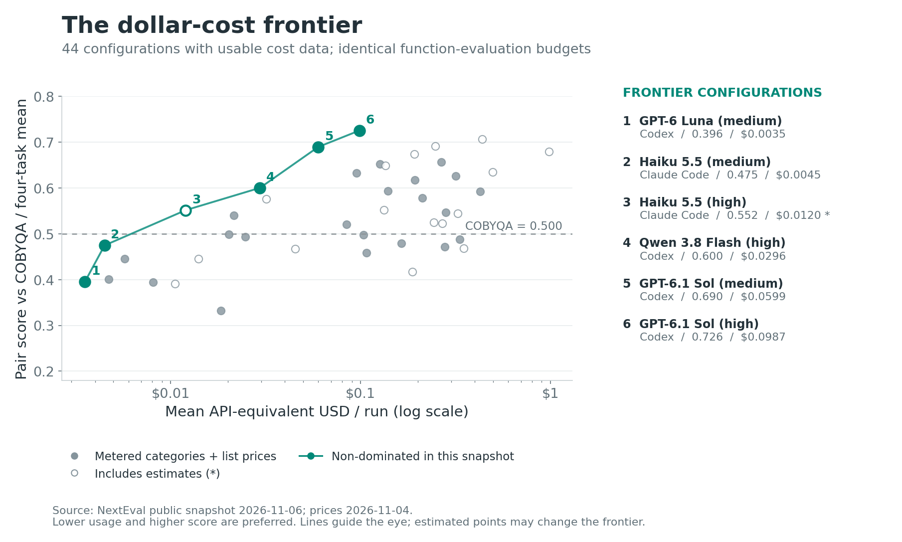
Four-task mean score against mean API-equivalent USD per run. Prices are dated November 4; hollow points include estimated usage. Interactive cost view.
GPT-6.1 Sol through Codex illustrates the trade-off. At medium effort, its mean score is 0.690 at $0.0599 per run; high effort gives 0.726 at $0.0987. The latter spends about 65% more for a 0.036 increase in the displayed score. That is a budget decision, and this small score gap alone does not establish a statistically reliable gain.
The frontier includes cheaper, lower-scoring options too. Being non-dominated means no displayed alternative is both cheaper and better-scoring; it does not mean the configuration clears a desired quality threshold. The dashed COBYQA line helps distinguish these questions. Of 45 displayed agent configurations, 44 have usable four-task cost data; 17 of those points include estimates.
2. Cheap in Dollars Does Not Mean Frugal in Tokens Link to heading
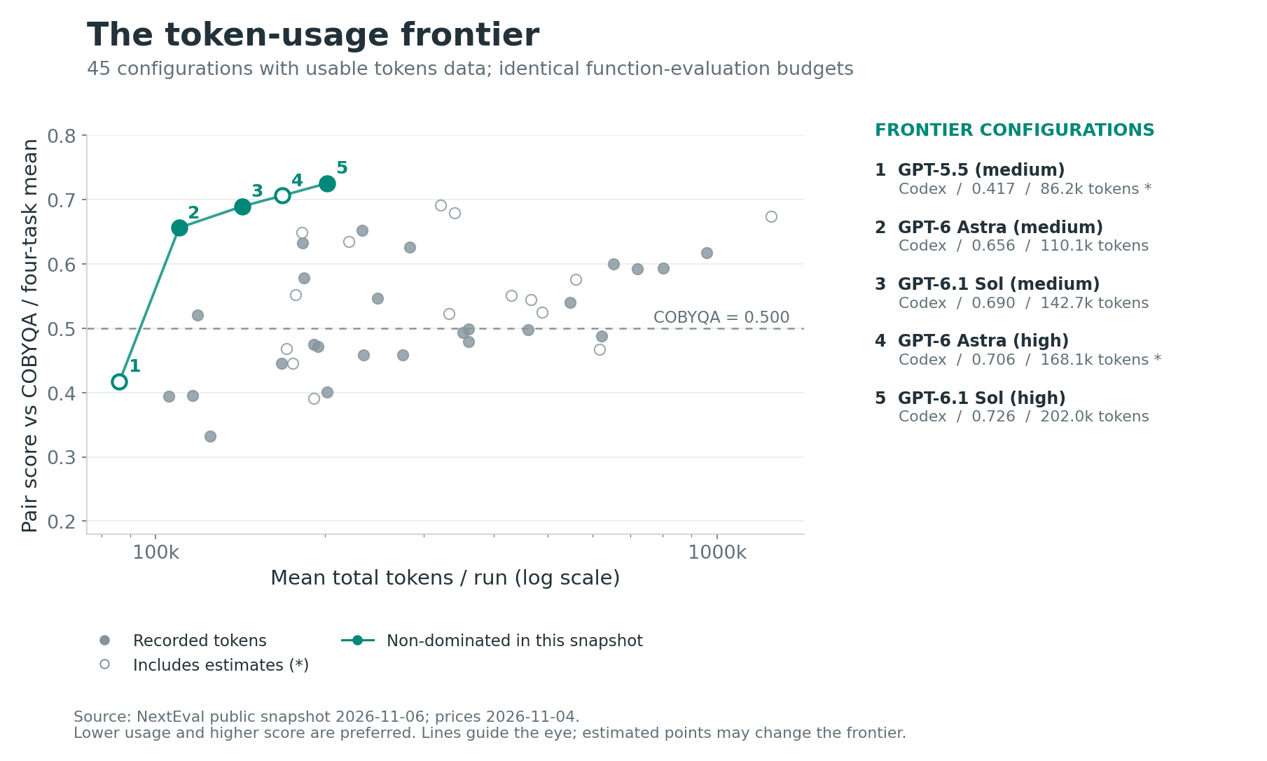
All 45 configurations have usable four-task token data; 17 points include estimates. Interactive token view.
Qwen 3.8 Flash (high) through Codex is on the dollar-cost frontier: about $0.0296 per run, with a mean score of 0.600. Yet it uses about 654k tokens per run. GPT-6.1 Sol (medium) uses about 143k, with a higher mean score of 0.690, so Qwen is not on the token frontier.
The two plots answer different questions. Prices and token categories affect dollar cost; token volume measures another aspect of resource use. For an optimization application, I would consider both alongside the objective-evaluation budget, rather than choosing from a score-only ranking. The plotted dollar costs are API-equivalent estimates from list prices, not bills.
3. Rotation Exposes a Shared Weakness Link to heading
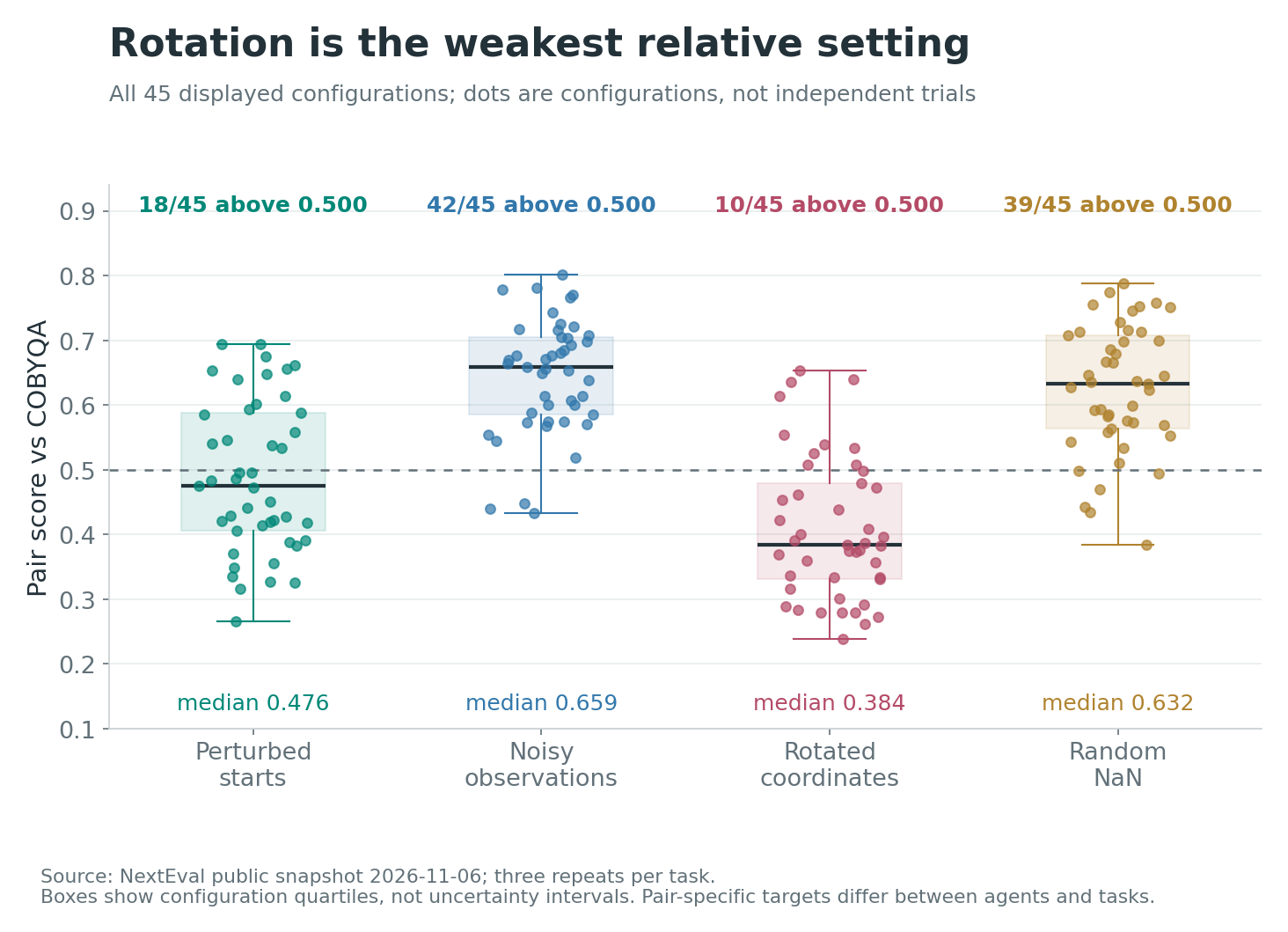
Each dot is a configuration, not an independent experimental repeat. Boxes summarize configuration quartiles. Task matrix.
Only 10 of 45 configurations score above 0.500 on rotated coordinates, compared with 42 of 45 on noisy observations. The corresponding medians are 0.384 and 0.659; perturbed starts and random NaN have medians of 0.476 and 0.632.
This makes rotation a useful diagnostic for the current systems: their relative position against COBYQA is often weaker when coordinate alignment changes. It motivates inspecting search-direction choices and local-model behavior. The plot does not identify the cause, and it does not show that noise makes optimization easier: each task uses its own agent–COBYQA comparisons and scoring targets.
4. Harness Choice Interacts with Model Choice Link to heading
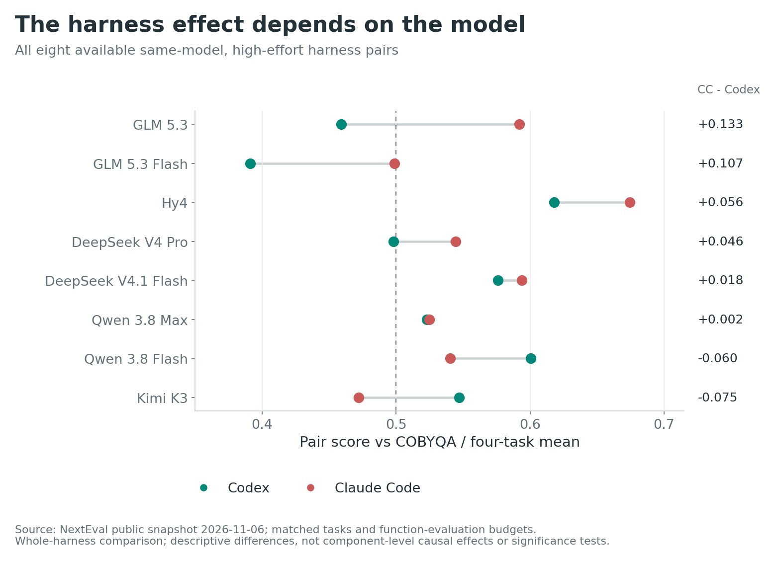
All eight available same-model, high-effort pairs; the right column is Claude Code minus Codex in four-task mean pair score.
GLM 5.3 moves from 0.459 in Codex to 0.592 in Claude Code, while Kimi K3 moves in the opposite direction, from 0.547 to 0.472. Qwen 3.8 Max is almost unchanged, at 0.523 and 0.525.
The practical implication is to evaluate the model–harness combination. The observed direction is not uniform across models. These are whole-system comparisons, including tool handling and conversation management; the chart neither isolates one harness component nor establishes significance for every gap.
5. A Strong Mean Still Contains Individual Losses Link to heading
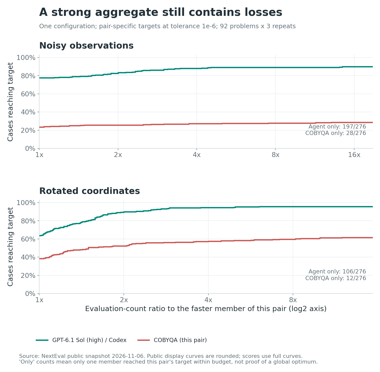
One configuration, selected because it has the highest four-task mean in this snapshot. Each panel has 276 cases and its own pair-specific targets at tolerance 1e-6. Inspect this agent.
On noisy observations, 197 cases reach the target only with the agent, while 28 reach it only with COBYQA. On rotated coordinates, those counts are 106 and 12. Thus, even the highest aggregate score leaves cases where the numerical baseline succeeds and the agent does not.
These profiles separate how quickly a target is reached from whether it is reached within the budget. That distinction directs the next investigation: inspect the histories of the COBYQA-only cases to look for premature stopping, unproductive method switches, or unsuitable search scales. The curves locate those questions; they do not establish a behavioral explanation without the traces.
NextEval Solver: Agent Decisions, Numerical Execution Link to heading
The NextEval Solver combines an LLM agent with a numerical environment. The agent selects tools, adjusts parameters, and assigns evaluation allowances. Numerical routines compute candidate points and evaluate the objective.
Tools support inspecting progress, fitting local models, and performing searches such as trust-region steps, polling, and line search. The environment maintains a shared evaluation history and each method’s numerical state. The agent can therefore change methods and later resume earlier work, with state checked and updated when needed.
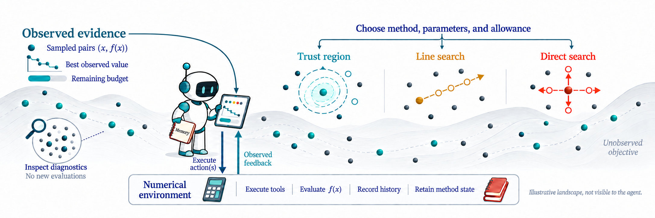
Overview from Figure 1 of our paper. The illustrated objective landscape is not visible to the agent.
What the Paper Establishes Link to heading
The paper reports improved function-evaluation efficiency against the tested classical baselines on its low-dimensional suite. It also studies model choice, reasoning settings, and execution harnesses through controlled comparisons. These are results for complete agent-and-tool systems; they do not isolate the LLM’s contribution or establish performance on unseen problem families.
The website continues to evolve beyond the paper’s experiment snapshot. In particular, its four-task, three-repeat protocol and current COBYQA pair score should be read using the website’s methodology, separately from the paper’s reported comparisons.
For me, NextEval connects two interests: building useful numerical optimization tools and understanding how agents make decisions from feedback. The Solver guide is a starting point for using the system; the Bench lets readers inspect the evidence.